10 Quads and Cubes
In this chapter we’re going to add two new kinds of primitives - quadrilaterals and cubes. We’ll also build a new scene with these primitives, i.e., the classic Cornel’s Box.
10.1 Theories
10.1.1 Quadraliterals
There’re multiple ways to represent a quad in graphics. What I’m using is to assume that a corner of the quad lies at the origin point. Then, two edges, \(\mathbf e_1\) and \(\mathbf e_2\), of the quad connected to this corner is used to define that quad. The normal could be find by the cross production of this two edge, i.e., The normal \(\mathbf n = \frac{\mathbf e_1 \times \mathbf e_2}{|\mathbf e_1 \times \mathbf e_2|}\), and this direction is the front of the quad.
Any point \(\mathbf p\) on that quad could be represented using \(\mathbf p = a \mathbf e_1 + b \mathbf e_2\), where \(a, b \in [0, 1]\). Along with the equation of ray, i.e., \(\mathbf p = \mathbf o + t \mathbf d, t \ge 0\), we can solve \(a\), \(b\) and \(t\) for later uasage. First, we rewrite the equation of the quad to an equation of the plane it lies on, \(\mathbf n \cdot \mathbf p = 0\). Now we can solve \(t\) as \(- \frac{\mathbf n \cdot \mathbf o}{\mathbf n \cdot \mathbf d}\). Then we can calculate the point \(\mathbf p\). Since point \(\mathbf p\) is on the plane, the equation
\[ E \binom{a}{b} = \mathbf p \]
could be used to solve \(a\) and \(b\). Where \(E\) is the matrix of composed of the vector \(\mathbf e_1\) and \(\mathbf e_2\)
\[ E = \left(\begin{array}{ll} e_{1 x} & e_{2 x} \\ e_{1 y} & e_{2 y} \\ e_{1 z} & e_{2 z} \end{array}\right) \]
Recall you linear algebra knowledge, the solution is
\[ \binom{a}{b} = E^+ \mathbf p \]
where \(E^+\) is the pseudo inverse of \(E\), i.e., \(E^+ = (E^T E)^{-1} E^T\).
10.1.2 Cubes
In our renderer, the cube will be defined using a vector \(\mathbf p\), and the formed cube is same as the AABB bounding box formed by the point \(\mathbf p\) and \(-\mathbf p\). The algorithm used for calculate ray-AABB intersection will be used for cubes.
We’ve calculated thw two parameter where the ray hits the AABB bounding box, so we can use them to calculate the two points on the cube. By comparing the component of this point and the bounding limit, we can know which side of the cube the point is on, and then it’s easy to know other information like the normal of the cube.
10.2 Implementation
Nothing special to design here. We just implement them as we’ve implemented the sphere.
10.2.1 Cube
The cube is defined as following:
We implement the Shape trait with the AABB bounding box where neessary methods are actually implemented before:
impl Shape for Cube {
    fn hit(&self, ray: Ray, rt_max: f32) -> Option<SurfaceHit> {
        if let Some((t1, t2)) = self.aabb.hit(ray, rt_max) {
            let t = if relative_eq!(t1, 0.0) { t2 } else { t1 };
            let hit_position = ray.origin + ray.direction * t;
            let normal = self.aabb.normal_at(hit_position);
            return Some(SurfaceHit::new(
                t,
                hit_position,
                normal.normalize(),
                ray.direction,
                self.material.clone(),
            ));
        }

        None
    }

    fn intersect(&self, ray: Ray, rt_max: f32) -> bool {
        self.aabb.ray_test(ray, rt_max)
    }

    fn aabb(&self) -> AABB {
        self.aabb
    }
}
The only special thing here is that we should check whether the origin of the ray is inside the cube or not. The implementation of AABB::ray_test will return 0 if the ray originates within the cube.
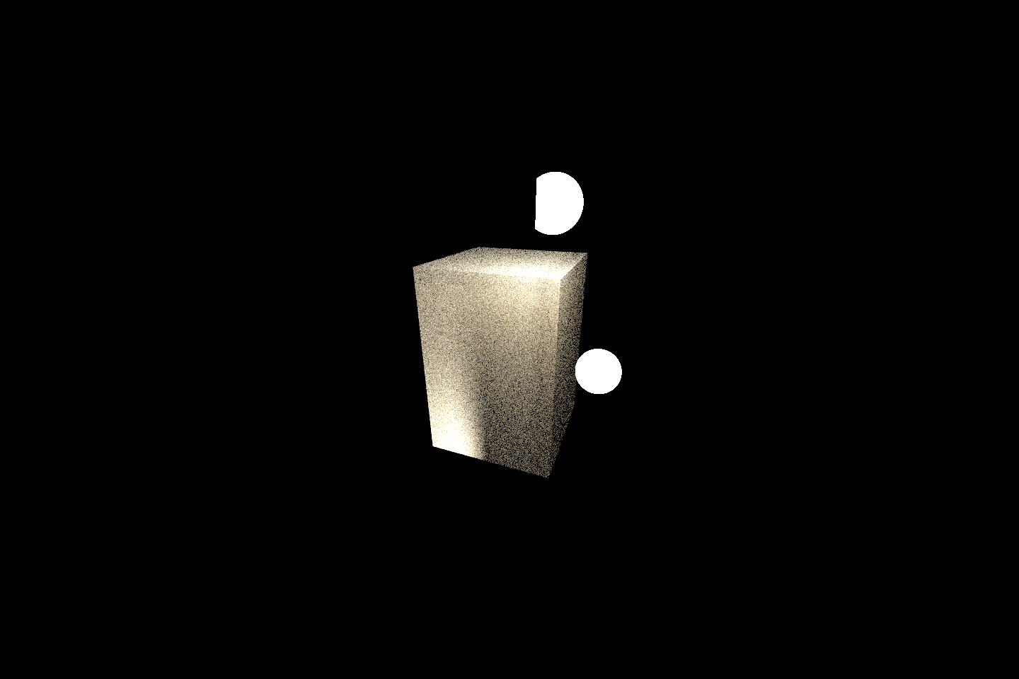
Here’s a simple scene with a cube:
10.2.2 Quads
As before, we can define the Quad struct easily:
#[derive(Debug, Clone)]
pub struct Quad {
    pub edges: (Vec3, Vec3),
    pub pseudo_inversion: (Vec3, Vec3),
    pub normal: Vec3,
    pub aabb: AABB,
    pub material: Arc<Material>,
}
Note that the normal and pseudo inersion of \(E\) are calculated in the constructor and saved.
impl Quad {
    // ...

    fn pseudo_inversion((e1, e2): (Vec3, Vec3)) -> (Vec3, Vec3) {
        // Compute elements of E^T * E
        let a11 = e1.length_squared();
        let a12 = e1.dot(e2);
        let a22 = e2.length_squared();

        // Determinant of the 2x2 matrix E^T * E
        let det = a11 * a22 - a12 * a12;

        // Compute the inverse of E^T * E
        let inv_a11 = a22 / det;
        let inv_a12 = -a12 / det;
        let inv_a22 = a11 / det;

        // Compute E^+ (pseudo-inverse of E)
        let row1 = inv_a11 * e1 + inv_a12 * e2;
        let row2 = inv_a12 * e1 + inv_a22 * e2;

        (row1, row2)
    }

    // ...
}
And most of the ray-quad inetersection are same for hit and intersect, so we can implement that in another method:
impl Quad {
    // ...

    fn ray_test(&self, ray: Ray, rt_max: f32) -> Option<(f32, f32, f32)> {
        let t = -self.normal.dot(ray.origin) / (self.normal.dot(ray.direction));
        if t < 0.001 || t > rt_max {
            return None;
        }
        let p = ray.evaluate(t);
        let a = self.pseudo_inversion.0.dot(p);
        let b = self.pseudo_inversion.1.dot(p);
        const RANGE: std::ops::RangeInclusive<f32> = 0.0..=1.0;
        if RANGE.contains(&a) && RANGE.contains(&b) {
            Some((t, a, b))
        } else {
            None
        }
    }
}
This is plain translation from our explanation above. With the three parameters, we can then implement the hit and intersect method easily, so they’re not included here. A note: when constructing the AABB bounding box for Quad, sometimes just add all four vertices together will be not enough - you may have an AABB with zero volume! So in my code, I expand that AABB a small value, so it’s not zero volume.
impl Quad {
    pub fn new(edges: (Vec3, Vec3), material: Arc<Material>) -> Self {
        let aabb = AABB::from_two_points(edges.0, edges.1)
            .add_point(Vec3::ZERO)
            .add_point(edges.0 + edges.1)
            .expand(0.01);

        // ...
    }

    // ...
}
And now we can build a simple Cornell Box scene to test our ray tracer! Mine looks like this:
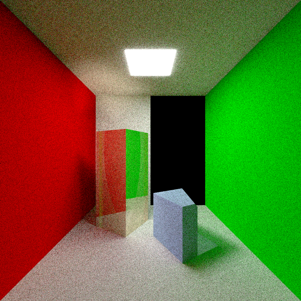
Experiement with this scene and make it more interesting.